A Bayesian network is a probabilistic model that represents a set of random variables and their conditional dependencies. They have extensive applications in areas such as
Pr(E|G) and innocent Pr(E|~G). But we need to infer the probability he's guilty given the evidence Pr(G|E).Pr(test|~disease) and Pr(~test|disease). But we need to infer the probability the patient has the disease given a positive test result Pr(disease|test).
- Many other diverse areas such as biology, sports betting, engineering and risk analysis.Judea Pearl, professor of computer science and statistics at UCLA, introduced the modern idea of a Bayesian net in his 1985 paper: Bayesian Networks: A Model of Self-Activated Memory for Evidential Reasoning.
Seventy two years prior, the US Jurist John Henry Wigmore developed an informal version of the Bayesian belief network for analyzing evidence in court trials in the June 1913 article "The problem of proof" found in the Illinois law review, Volume 8 Number 2, pp. 77-103. Wigmore charts are still used to this day by lawyers to analyze evidence in court cases.
Harvard Professor Joel Blitzstein said, "The soul of statistics is conditioning." The precise mathematical method for "inverting" a conditional probability to determine the probability of an unobserved variable is Bayes Law, developed by the Reverend Thomas Bayes in his Essay towards solving a Problem in the Doctrine of Chances in 1763.
More than two millenium prior, the rhethoritician Gorgias (483—375 B.C.E.) presented the archetype of a legal argument based on the conditional probabilities connecting evidence to guilt. This speech is entitled The Defense of Palamedes. I have an essay on it: On Gorgias' Defense of Palamedes. The centrality of Palamedes in this seminal work is yet another important reason this software bears his name!
For modern, up-to-date approaches to graphically analyzing legal arguments using Bayesian networks, see
One motivation for automating Bayesian inference is that many people find it difficult to reason about conditional probabilities, and there are many common fallacies. Two prominent fallacies are
Pr(A|B) ≈ Pr(B|A). Example: "Terrorists tend to have an engineering background; so, engineers have a tendency towards terrorism."In the paper Probabilistic reasoning in clinical medicine: Problems and opportunities by David M. Eddy (1982), a hundred physicians were asked about the probability of having a disease based on a positive test result; 95% of these doctors committed the inverse fallacy in their answer. The Sally Clark case is a recent example of an expert witness committing the prosecutor's fallacy. See
Palamedes allows a user to input relationships among a set of random variables. It then can answer probabilistic queries about them.
Right now, Palamedes' Bayes net model only supports binary random variables, e.g., guilty and ~guilty (meaning "not guilty" or "innocent"). In a future version, random variables will be able to take arbitrary values, e.g., Weather=snow, Weather=rain, or Weather=sunny.
Probabilities are input or queried into the system via statements of the form Pr(Conjunction1 of random variables | Conjunction2 of random variables). The bar | (meaning "given") and the second conjunction are optional. Here are a few examples:
| Command | Notes |
|---|---|
Pr(guilty) gets value0 | Example of inputting an unconditional probability |
Pr(evidence1|~guilty) gets value1 | Example of inputting a conditional probability |
Pr(guilty|evidence1,evidence2,evidence3) | Example of querying a conditional probability involving a conjunction of random variables |
Conjunctions between random variables may be input using commas; the word "and" or the symbol &&; or the word "intersect" or the symbol ∩.
Exact and approximate methods exist for inferring unobserved variables in Bayesian networks. Common exact methods include exponential enumeration and variable elimination. Approximate methods include importance sampling, belief propagation, and stochastic MCMC simulation.
Palamedes uses an exact method that takes an AI/logic programming approach. It uses pattern matching to match user inputs against mathematical rules for making deductions until the current goal is achieved. The rules are simply what you would find in any probability and statistics textbook about conditional probabilities:
Pr(A∩B) = PR(A|B)*Pr(B)Pr(~A) = 1 - Pr(A)Pr(A|B) = Pr(B|A)*Pr(A)/Pr(B)Pr(A|B) = Pr(A|B∩C)*Pr(C) + Pr(A|B∩~C)*Pr(~C)To see a table of all of the deductions made by the system, use the command bayes(). Note: These deductions are memoized. If you need to clear them because you've added new info or changed values, simply pass an argument to the bayes function, e.g., bayes(0).
This implementation is inspired by Ivan Bratko's interpreter for belief networks, figure 15.11, in the book Prolog Programming for Artificial Intelligence. It has comparable performance to variable elimination.
Palamedes is one of many software applications available for Bayesian analysis.
There are two main groups of alternative software:
As a Bayesian calculator, Palamedes doesn't have graphical input or output. Its main limitation stems from the exact inference method it implements, which has computational complexity O(k*2^k). Approximate methods are needed to deal with large belief networks. In a future version, Palamedes will implement an MCMC method for dealing with large nets. Currenty, Palamedes only supports binary random variables, another limitation that will get relaxed in a future version.
As a Bayesian calculator, Palamedes still has several advantages. The input uses the same syntax you might see in a math textbook. And it will actually show you the derivations it made to reach its conclusions if you call the bayes() function. That's because the algorithm it uses is a rule-based AI system.
But Palamedes doesn't focus on being merely a Bayesian inference engine. It also has a dice roller similar to Troll. And it has many built-in probability and statistics functions, though nothing like R. It can even be used as a desktop calculator. And in the future, it will get computer algebra capabilities.
Additionally, Palamedes is Turing Complete. The language itself is array-based, rather like APL, though nowhere near as cryptic hopefully. It's as easy to manipulate an array or matrix as it is to manipulate a number.
Palamedes' main advantage is that it is written in pure JavaScript, so it runs in a web browser or at a command-prompt using Node.js. It is 100% free and open-source. And it has a relatively small footprint, only a couple hundred KB as opposed to 11.5-13.0MB for OpenBUGS or OpenMarkov.
The following example of legal reasoning in a court case example comes from the paper Teaching an Application of Bayes' Rule for Legal Decision-Making: Measuring the Strength of Evidence, pp. 10-12.
| Command | Results |
|---|---|
/* 3.1.1 Calculation of Posterior Probability after Evidence 1 (E₁), p. 10 */ Pr( G) ← 0.5 Pr(~G) NB. Should be 0.5 Pr(E₁|G) ← 1 Pr(E₁|~G) ← 0.45 Pr(G|E₁) NB. Should be 0.69 /* 3.2.1 Calculation of Posterior Probability after the Second Piece of Evidence (E₂), p. 11 */ Pr(~G|E₁) NB. Should be 0.31 Pr(E₂|G and E₁) ← 1 Pr(E₂|~G and E₁) ← 0.21 Pr(G|E₁ and E₂) NB. Should be 0.914 /* 3.3.1 Calculation of Posterior Probability after Evidence 3 (E₃), p. 12 */ Pr(~G|E₁ and E₂) NB. Should be 0.086 Pr(E₃|G and E₁ and E₂) ← 1 Pr(E₃|~G and E₁ and E₂) ← 0.017 Pr(G|E₁ and E₂ and E₃) NB. Should be 0.998 | Pr(G) ← 0.5 Pr(~G) → 0.5 Pr(E₁ | G) ← 1 Pr(E₁ | ~G) ← 0.45 Pr(G | E₁) → 0.6896551724137931 Pr(~G | E₁) → 0.31034482758620685 Pr(E₂ | E₁ ∩ G) ← 1 Pr(E₂ | E₁ ∩ ~G) ← 0.21 Pr(G | E₁ ∩ E₂) → 0.9136592051164916 Pr(~G | E₁ ∩ E₂) → 0.08634079488350843 Pr(E₃ | E₁ ∩ E₂ ∩ G) ← 1 Pr(E₃ | E₁ ∩ E₂ ∩ ~G) ← 0.017 Pr(G | E₁ ∩ E₂ ∩ E₃) → 0.998396076702777 |
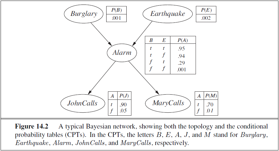
The following example comes from Figure 14.2 on page 512 in the book Artificial Intelligence: A Modern Approach by Stuart Russell and Peter Norvig.
| Command | Results |
|---|---|
/* Input probability tables */ Pr(JohnCalls| Alarm) gets 0.90 Pr(JohnCalls|~Alarm) gets 0.05 Pr(MaryCalls| Alarm) gets 0.70 Pr(MaryCalls|~Alarm) gets 0.01 Pr(Alarm| Burglary and Earthquake) gets 0.95 Pr(Alarm| Burglary and ~Earthquake) gets 0.94 Pr(Alarm|~Burglary and Earthquake) gets 0.29 Pr(Alarm|~Burglary and ~Earthquake) gets 0.001 Pr(Burglary) gets 0.001 Pr(Earthquake) gets 0.002 /* Query the system */ Pr(JohnCalls, MaryCalls, Alarm, ~Burglary, ~Earthquake) NB. Should be 0.000628 Pr(Burglary | JohnCalls, MaryCalls) NB. Should be 0.28 | Pr(JohnCalls | Alarm) ← 0.90 Pr(JohnCalls | ~Alarm) ← 0.05 Pr(MaryCalls | Alarm) ← 0.70 Pr(MaryCalls | ~Alarm) ← 0.01 Pr(Alarm | Burglary ∩ Earthquake) ← 0.95 Pr(Alarm | Burglary ∩ ~Earthquake) ← 0.94 Pr(Alarm | Earthquake ∩ ~Burglary) ← 0.29 Pr(Alarm | ~Burglary ∩ ~Earthquake) ← 0.001 Pr(Burglary) ← 0.001 Pr(Earthquake) ← 0.002 Pr(Alarm ∩ JohnCalls ∩ MaryCalls ∩ ~Burglary ∩ ~Earthquake) → 0.0006281112599999999 Pr(Burglary | JohnCalls ∩ MaryCalls) → 0.28417183536439294 |
In order to see the deductions made by the system in Example 2, use the bayes() command. You'll see the following table:
bayes() →
                                                         key     value
    Alarm ∩ JohnCalls ∩ MaryCalls ∩ ~Burglary ∩ ~Earthquake|     Pr(JohnCalls) * Pr(Alarm ∩ MaryCalls ∩ ~Burglary ∩ ~Earthquake | JohnCalls)
       Alarm ∩ MaryCalls ∩ ~Burglary ∩ ~Earthquake|JohnCalls     Pr(MaryCalls | JohnCalls) * Pr(Alarm ∩ ~Burglary ∩ ~Earthquake | JohnCalls ∩ MaryCalls)
       Alarm ∩ ~Burglary ∩ ~Earthquake|JohnCalls ∩ MaryCalls     Pr(Alarm | JohnCalls ∩ MaryCalls) * Pr(~Burglary ∩ ~Earthquake | Alarm ∩ JohnCalls ∩ MaryCalls)
                                                      Alarm|     Pr(Alarm | Burglary ∩ Earthquake) * Pr(Burglary ∩ Earthquake) + Pr(Alarm | Burglary ∩ ~Earthquake) * Pr(Burglary ∩ ~Earthquake) + Pr(Alarm | Earthquake ∩ ~Burglary) * Pr(Earthquake ∩ ~Burglary) + Pr(Alarm | ~Burglary ∩ ~Earthquake) * Pr(~Burglary ∩ ~Earthquake)
                                      Alarm|Alarm ∩ Burglary     1
                                     Alarm|Alarm ∩ JohnCalls     1
                         Alarm|Alarm ∩ JohnCalls ∩ ~Burglary     1
           Alarm|Alarm ∩ JohnCalls ∩ ~Burglary ∩ ~Earthquake     1
                                     Alarm|Alarm ∩ ~Burglary     1
                       Alarm|Alarm ∩ ~Burglary ∩ ~Earthquake     1
                                              Alarm|Burglary     Pr(Alarm | Burglary ∩ Earthquake) * Pr(Burglary ∩ Earthquake | Burglary) + Pr(Alarm | Burglary ∩ ~Earthquake) * Pr(Burglary ∩ ~Earthquake | Burglary) + Pr(Alarm | Earthquake ∩ ~Burglary) * Pr(Earthquake ∩ ~Burglary | Burglary) + Pr(Alarm | ~Burglary ∩ ~Earthquake) * Pr(~Burglary ∩ ~Earthquake | Burglary)
                                 Alarm|Burglary ∩ Earthquake     0.95
                                  Alarm|Burglary ∩ JohnCalls     Pr(Alarm | Burglary) * Pr(JohnCalls | Alarm ∩ Burglary) / Pr(JohnCalls | Burglary)
                                Alarm|Burglary ∩ ~Earthquake     0.94
                                Alarm|Earthquake ∩ ~Burglary     0.29
                                             Alarm|JohnCalls     Pr(Alarm) * Pr(JohnCalls | Alarm) / Pr(JohnCalls)
                                 Alarm|JohnCalls ∩ MaryCalls     Pr(Alarm | JohnCalls) * Pr(MaryCalls | Alarm ∩ JohnCalls) / Pr(MaryCalls | JohnCalls)
                                             Alarm|~Burglary     Pr(Alarm | Burglary ∩ Earthquake) * Pr(Burglary ∩ Earthquake | ~Burglary) + Pr(Alarm | Burglary ∩ ~Earthquake) * Pr(Burglary ∩ ~Earthquake | ~Burglary) + Pr(Alarm | Earthquake ∩ ~Burglary) * Pr(Earthquake ∩ ~Burglary | ~Burglary) + Pr(Alarm | ~Burglary ∩ ~Earthquake) * Pr(~Burglary ∩ ~Earthquake | ~Burglary)
                               Alarm|~Burglary ∩ ~Earthquake     0.001
                                      Burglary ∩ Earthquake|     Pr(Burglary) * Pr(Earthquake | Burglary)
                              Burglary ∩ Earthquake|Burglary     Pr(Burglary | Burglary) * Pr(Earthquake | Burglary)
                             Burglary ∩ Earthquake|~Burglary     Pr(Burglary | ~Burglary) * Pr(Earthquake | Burglary ∩ ~Burglary)
                                     Burglary ∩ ~Earthquake|     Pr(Burglary) * Pr(~Earthquake | Burglary)
                             Burglary ∩ ~Earthquake|Burglary     Pr(Burglary | Burglary) * Pr(~Earthquake | Burglary)
                            Burglary ∩ ~Earthquake|~Burglary     Pr(Burglary | ~Burglary) * Pr(~Earthquake | Burglary ∩ ~Burglary)
                                                   Burglary|     0.001
                                           Burglary|Burglary     1
                                          Burglary|JohnCalls     Pr(Burglary) * Pr(JohnCalls | Burglary) / Pr(JohnCalls)
                              Burglary|JohnCalls ∩ MaryCalls     Pr(Burglary | JohnCalls) * Pr(MaryCalls | Burglary ∩ JohnCalls) / Pr(MaryCalls | JohnCalls)
                                          Burglary|~Burglary     0
                                     Earthquake ∩ ~Burglary|     Pr(~Burglary) * Pr(Earthquake | ~Burglary)
                             Earthquake ∩ ~Burglary|Burglary     Pr(~Burglary | Burglary) * Pr(Earthquake | Burglary ∩ ~Burglary)
                            Earthquake ∩ ~Burglary|~Burglary     Pr(~Burglary | ~Burglary) * Pr(Earthquake | ~Burglary)
                                                 Earthquake|     0.002
                                         Earthquake|Burglary     Pr(Earthquake)
                             Earthquake|Burglary ∩ ~Burglary     Pr(Earthquake)
                                        Earthquake|~Burglary     1 - Pr(~Earthquake | ~Burglary)
                                                  JohnCalls|     Pr(JohnCalls | Alarm) * Pr(Alarm) + Pr(JohnCalls | ~Alarm) * Pr(~Alarm)
                                             JohnCalls|Alarm     0.90
                                  JohnCalls|Alarm ∩ Burglary     Pr(JohnCalls | Alarm) * Pr(Alarm | Alarm ∩ Burglary) + Pr(JohnCalls | ~Alarm) * Pr(~Alarm | Alarm ∩ Burglary)
                                 JohnCalls|Alarm ∩ ~Burglary     Pr(JohnCalls | Alarm) * Pr(Alarm | Alarm ∩ ~Burglary) + Pr(JohnCalls | ~Alarm) * Pr(~Alarm | Alarm ∩ ~Burglary)
                   JohnCalls|Alarm ∩ ~Burglary ∩ ~Earthquake     Pr(JohnCalls | Alarm) * Pr(Alarm | Alarm ∩ ~Burglary ∩ ~Earthquake) + Pr(JohnCalls | ~Alarm) * Pr(~Alarm | Alarm ∩ ~Burglary ∩ ~Earthquake)
                                          JohnCalls|Burglary     Pr(JohnCalls | Alarm) * Pr(Alarm | Burglary) + Pr(JohnCalls | ~Alarm) * Pr(~Alarm | Burglary)
                                            JohnCalls|~Alarm     0.05
                                             MaryCalls|Alarm     0.70
                                 MaryCalls|Alarm ∩ JohnCalls     Pr(MaryCalls | Alarm) * Pr(Alarm | Alarm ∩ JohnCalls) + Pr(MaryCalls | ~Alarm) * Pr(~Alarm | Alarm ∩ JohnCalls)
                     MaryCalls|Alarm ∩ JohnCalls ∩ ~Burglary     Pr(MaryCalls | Alarm) * Pr(Alarm | Alarm ∩ JohnCalls ∩ ~Burglary) + Pr(MaryCalls | ~Alarm) * Pr(~Alarm | Alarm ∩ JohnCalls ∩ ~Burglary)
       MaryCalls|Alarm ∩ JohnCalls ∩ ~Burglary ∩ ~Earthquake     Pr(MaryCalls | Alarm) * Pr(Alarm | Alarm ∩ JohnCalls ∩ ~Burglary ∩ ~Earthquake) + Pr(MaryCalls | ~Alarm) * Pr(~Alarm | Alarm ∩ JohnCalls ∩ ~Burglary ∩ ~Earthquake)
                              MaryCalls|Burglary ∩ JohnCalls     Pr(MaryCalls | Alarm) * Pr(Alarm | Burglary ∩ JohnCalls) + Pr(MaryCalls | ~Alarm) * Pr(~Alarm | Burglary ∩ JohnCalls)
                                         MaryCalls|JohnCalls     Pr(MaryCalls | Alarm) * Pr(Alarm | JohnCalls) + Pr(MaryCalls | ~Alarm) * Pr(~Alarm | JohnCalls)
                                            MaryCalls|~Alarm     0.01
                                                     ~Alarm|     1 - Pr(Alarm)
                                     ~Alarm|Alarm ∩ Burglary     0
                                    ~Alarm|Alarm ∩ JohnCalls     0
                        ~Alarm|Alarm ∩ JohnCalls ∩ ~Burglary     0
          ~Alarm|Alarm ∩ JohnCalls ∩ ~Burglary ∩ ~Earthquake     0
                                    ~Alarm|Alarm ∩ ~Burglary     0
                      ~Alarm|Alarm ∩ ~Burglary ∩ ~Earthquake     0
                                             ~Alarm|Burglary     1 - Pr(Alarm | Burglary)
                                 ~Alarm|Burglary ∩ JohnCalls     1 - Pr(Alarm | Burglary ∩ JohnCalls)
                                            ~Alarm|JohnCalls     1 - Pr(Alarm | JohnCalls)
                                    ~Burglary ∩ ~Earthquake|     Pr(~Burglary) * Pr(~Earthquake | ~Burglary)
       ~Burglary ∩ ~Earthquake|Alarm ∩ JohnCalls ∩ MaryCalls     Pr(~Burglary | Alarm ∩ JohnCalls ∩ MaryCalls) * Pr(~Earthquake | Alarm ∩ JohnCalls ∩ MaryCalls ∩ ~Burglary)
                            ~Burglary ∩ ~Earthquake|Burglary     Pr(~Burglary | Burglary) * Pr(~Earthquake | Burglary ∩ ~Burglary)
                           ~Burglary ∩ ~Earthquake|~Burglary     Pr(~Burglary | ~Burglary) * Pr(~Earthquake | ~Burglary)
                                                  ~Burglary|     1 - Pr(Burglary)
                                             ~Burglary|Alarm     Pr(~Burglary) * Pr(Alarm | ~Burglary) / Pr(Alarm)
                                 ~Burglary|Alarm ∩ JohnCalls     Pr(~Burglary | Alarm) * Pr(JohnCalls | Alarm ∩ ~Burglary) / Pr(JohnCalls | Alarm)
                     ~Burglary|Alarm ∩ JohnCalls ∩ MaryCalls     Pr(~Burglary | Alarm ∩ JohnCalls) * Pr(MaryCalls | Alarm ∩ JohnCalls ∩ ~Burglary) / Pr(MaryCalls | Alarm ∩ JohnCalls)
                                          ~Burglary|Burglary     0
                                         ~Burglary|~Burglary     1
       ~Earthquake|Alarm ∩ JohnCalls ∩ MaryCalls ∩ ~Burglary     Pr(~Earthquake | Alarm ∩ JohnCalls ∩ ~Burglary) * Pr(MaryCalls | Alarm ∩ JohnCalls ∩ ~Burglary ∩ ~Earthquake) / Pr(MaryCalls | Alarm ∩ JohnCalls ∩ ~Burglary)
                   ~Earthquake|Alarm ∩ JohnCalls ∩ ~Burglary     Pr(~Earthquake | Alarm ∩ ~Burglary) * Pr(JohnCalls | Alarm ∩ ~Burglary ∩ ~Earthquake) / Pr(JohnCalls | Alarm ∩ ~Burglary)
                               ~Earthquake|Alarm ∩ ~Burglary     Pr(~Earthquake | ~Burglary) * Pr(Alarm | ~Burglary ∩ ~Earthquake) / Pr(Alarm | ~Burglary)
                                        ~Earthquake|Burglary     1 - Pr(Earthquake | Burglary)
                            ~Earthquake|Burglary ∩ ~Burglary     1 - Pr(Earthquake | Burglary ∩ ~Burglary)
                                       ~Earthquake|~Burglary     1 - Pr(Earthquake)
To clear these deductions, use the command bayes(0).
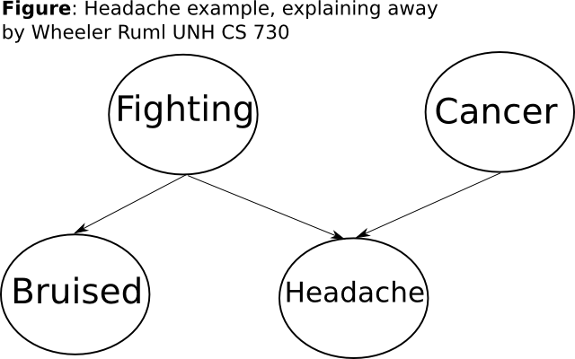
This example comes from an AI Lecture on YouTube about Bayesian networks, namely UNH CS 730 by Wheeler Ruml. Here is a diagram:
And here is the corresponding Palamedes code:
/* Bayes net headache example, explaining away by Wheeler Ruml UNH CS 730 */
/* https://www.youtube.com/watch?v=uM34RlzxfOk */
/* Note that "F" stands for Fudge dice in Palamedes, so we spell out the random variable "Fighting" */
Pr(Fighting) gets 0.02
Pr(Cancer) gets 0.1
Pr(Bruised|Fighting) gets 0.9
Pr(Bruised|~Fighting) gets 0.001
Pr(Headache|Fighting,Cancer) gets 0.99
Pr(Headache|Fighting,~Cancer) gets 0.9
Pr(Headache|~Fighting,Cancer) gets 0.75
Pr(Headache|~Fighting,~Cancer) gets 0.05
Pr(Cancer|Headache) NB. about 0.5525 from video at 16 min 34 sec
Pr(Cancer|Headache,Bruised) NB. about 0.112 from video at 26 min 27 sec
The system responds with the correct answers:
Pr(Cancer | Headache) → 0.5558992487847989
Pr(Cancer | Bruised ∩ Headache) → 0.11259375227554067
Last update: Fri Sep 23 2016