1 Introduction

In the thread Non-Linear Randomly-Generated Dungeon, thecoldironkid wrote:

For my game, I am attempting to write a series of dungeon tables (somewhat like Appendix A in the DMG, but tailored to my own material) so that I can generate game content randomly, at the table, on the fly.

As an aside: DMG Appendix A largely reproduces material from the article “Solo Dungeon Adventures” by EGG in The Strategic Review Vol. 1 No. 1 Spring 1975, which appears in the thread Gygax OD&D Additions.

thecoldironkid continues:

However, what I’ve come up with (like the tables in the DMG) can only produce endlessly-branching nodes without making explicit provision for “loops” or a “jacquayed dungeon” or whatever you want to call it. Is the only way to achieve a more complex, interconnected dungeon in this manner to wait for the ever-expanding map to just run into itself, and then decree, “Yup, this is where the loop is”? Maybe someone here has some insight into this that I’m missing?

Yes, this mechanism produces “dendritic” dungeons, rather than lairs with loops or meandering mazes. This, I argue below, is a good thing, because most natural cave systems have this branchwork pattern.

If you want a different dungeon topology, then you need a different mechanism.

In the thread on flow-chart style mapping for the DM too, I wrote several posts about using graphs as dungeon maps.

Below, I’m going to present three different graph-based mechanisms for generating dungeons, each one targeting a different topology:

1. loopy lairs
2. meandering mazes
3. (dimensionally dependable) dendritic dungeons

A graph is just a set of vertices (aka nodes) and edges connecting them. In a planar graph, the edges divide the plane up into faces (aka regions). At the bottom of this post, I provide an appendix with a crash course on graphs that explains this terminology in more detail. Here’s how I interpret what “vertex” and “edge” and “face” mean in each context:

1. In a lair with loops, a vertex represents either a room or some other interesting area on the map. An edge connects these areas. Its an “exit” – it could be an archway, a portcullis, a wooden door, a locked iron door, a secret door, a trap door, a teleportation device, a wormhole; or it could be a twisty passage, a hallway with a corner, a bridge, a long straight sloped narrow tunnel,… in short, any way to get from one area to another. A face is just the solid wall or rock separating areas.
2. In a meandering maze, a face represents a room/region/area, and an edge represents a wall. (Vertices merely represent junction points where walls come together.)
3. In a dendritic dungeon, a vertex represents a cavern and edges just show how they’re connected.

2 Loopy Lairs

In this section, I’m going to explain how I’d tackle the problem of generating dungeons with loops. This section is subdivided into two parts:

1. The Erdős-Rényi Model: A naïve method. Easy to understand. Simple to perform. But it doesn’t scale well for large dungeons. And it produces dungeons with properties that may be undesirable.
2. The Five Room Dungeon Model: My preferred method. Works by using a d20 roll and a table lookup, just like DMG Appendix A. One iteration only produces a small graph corresponding to a five room dungeon. But the method may be applied recursively, in order to produce bigger and bigger dungeons.

2.1 The Erdős-Rényi Model

Here’s a naïve method for randomly generating a dungeon from a graph:

1. Grab an \(N\)-sided die.
2. Grab a piece of graph paper and a pencil.
3. Randomly dot the paper \(N\) times and label these dots \(1, 2, \ldots, N\). These dots are called vertices.
4. Next roll your d\(N\) twice, to produce two numbers \(X\) and \(Y\).
5. Draw an edge from vertex \(X\) to vertex \(Y\).
6. Repeat steps (4)-(5) \(M\) times. You want to make \(M\) big enough so that your graph has the desired topological properties – connectedness, cycles, etc. But you want \(M\) small enough so that the resulting graph doesn’t look like a “hairball” – a big mess.
7. Now interpret each vertex as a room or other interesting area on your map; and interpret each edge as an “exit” such as a door or corridor, leading to another area.

This method is very easy to perform but lacks sophistication. Theoretically, you could randomly generate any graph with \(N\) vertices and \(M\) edges, just as if you took them all, put them into a hat, shook it around, and pulled out one at random. This model for generating random graphs is called the Erdős-Rényi Model.

But there are some issues with this method:

• If you start with a big \(N\), say \(N=20\), then you are going to need a suitably big \(M\), maybe \(M=50\), to get a graph with that’s connected and has cycles. That means rolling 100 times to generate the edges! That’s easy enough to do on a computer, but it’s not something you can easily do on-the-fly at the game table.
• There’s no guarantee that the resulting graph is planar – one that may be drawn in a plane with no edge crossings.
• The degree distribution (probability that a vertex has so many incident edges) follows a Poisson Distribution. That’s not how real-life networks (like cave systems, streams, your circulatory system, trade networks in free markets, facebook or the internet) behave – the degree distribution of those graphs follows a Power Law. A power law distribution looks like \(f(x) \propto x^{-\gamma}\). This distribution only has a well-defined mean if \(\gamma > 2\), and it only has a finite variance if \(\gamma > 3\).

If you want a fast, automated way to generate Erdős-Rényi random graphs, then you might use WolframAlpha, a free online “computaional knowledge engine.” Here’s a sample query that produces a random graph with 10 vertices and 25 edges.

2.2 The Five Room Dungeon Model

In Roleplaying Tips #156, Johnn Four presents his Five Room Dungeon Model. I like that model. I’m not going to rehash it here. But I find it easy to create dungeons on-the-fly in five room “chunks.”

As good fortune would have it, there are exactly 20 nonisomorphic simple connected planar 5-graphs! So the first step is to roll a d20 on the following table, in order to determine the topology of the next five-room hunk of the dungeon:

Graph Type

d20 Die Roll	Graph Name	Graph Image
1	bull
2	butterfly/hourglass
3	\(C_5\) (cycle)
4	co-fork
5	co-P
6	cricket
7	dart
8	fork/chair
9	gem
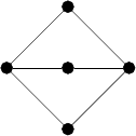
10	house
11	\(K_{1,4}\)
12	\(K_{2,3}\)
13	\(K_5 - e\)
14	\(\overline{\text{claw} \cup K_1}\)
15	\(\overline{K_3 \cup 2 K_1}\)
16	\(\overline{P_2 \cup P_3}\)
17	\(\overline{P_3 \cup 2 K_1}\)
18	P
19	\(P_5\) (path)
20	\(W_4\) (wheel)

All we’ve done so far is to determine the topology of this part of the dungeon. Topology is not the same geometry. Topology just tells us how our five rooms are wired together – not about their sizes, their shapes, or even their relative positions!

One way to determine room size and shape would be to cut various shapes and sizes out of cardboard, stick them in a hat, sack or bag, and pick them out at random when you need them.

An alternative method would be to roll dice and use a lookup table.

Whichever method you use, feel free to “overrule” any random results and replace them with your own judgment or cool feature that just popped into mind.

The following tables may be used to determine room size, shape and exit types. Note that you do not need to roll in advance for all five rooms – you only need to roll for the areas your players are actively exploring!

(As an aside, sometimes room shape suggests the contents: A hexagonal room suggests honeycombs with giant bees. A pentagram-shaped room suggests robed Satanists, a sacrificial altar and a giant statue of Baphomet.)

Relative room positions: As you assign sizes and shapes to the five rooms, you may need to “push them apart” so that they’ll fit on your map. Keep your descriptions consistent with what you’ve already told the players. But you’re free to rotate or translate the unexplored graph vertices and edges. Just avoid edge crossings.

Since the topology doesn’t tell us what kind of “exit” an edge represents, here is a table to determine the nature of each edge/connection in the graph:

The topology doesn’t tell us the exact location of these exits. Best to judge this on a case-by-case basis, based on relative room positioning.

As your players explore each area of the map, you’ll also need to fill each room with monsters, treasures, traps and other features. I’m not providing tables for that… For monsters and treasure, I use the Distribution of Monsters and Treasure rules on pages 6-8 of U&WA/Vol. 3. This in turn uses the MONSTER DETERMINATION AND LEVEL OF MONSTER MATRIX on pages 10-11 of U&WA/Vol. 3. For traps, use TABLE VII. TRICK/TRAP in the aforementioned “SOLO DUNGEON ADVENTURES” article.

2.2.1 Example: Translating the House Graph into a Five Room Dungeon

I have implemented these tables in Palamedes, the online dice roller and probability calculator I developed. The script is here. You can run it with this link. And here is a screenshot of the output.

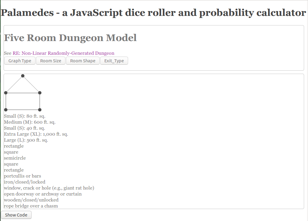
So first I generated the Graph Type and got a House Graph. Next I clicked Room Size 5 times, then Room Shape 5 times. Finally I clicked Exit Type 6 times, since this graph has 6 edges.

And here is how I translated these results into a map:

Then I applied Johnn Four’s Five Room Dungeon Model to flesh it out a little:

1. Entrance And Guardian. Medium (L): 500 ft. sq. Shape: rectangle about 45'10" x 10'11.5". This is the entrance to the dungeon. On the S wall of the room to your right as you enter is a closed wooden door. On the S wall to your left as you enter you can see a room filled with exquiste treasures: gold, jewels, weapons. But a set of iron bars deny you entrance to this room. There’s another party of adventurers trying in vain to hack their way through the bars. One of them turns your way, sneers at you, and says: “GTFO now or die!” DM only: The bars only open from the other side!
2. Puzzle Or Roleplaying Challenge. Extra Large (XL): 1,000 ft. sq. Shape: square about 31'7" x 31'7". There is a closed locked iron door on the E wall near the N corner (the key is in room 4). Most of the E side of this room has a deep chasm running N-S, due to cave-ins or collapse. The chasm is about 10' across. There is a rope bridge across the chasm near the SE corner. DM only: This chamber is collapsing, creating a death trap! Imagine an 8x8 chessboard-like grid overlaying it (see map). If the players step on a “black” square (marked with an X), it immediately collpases. Make a saving throw or suffer d6 damage. Plus it takes time to climb out. If the players map this out, they will realize it is a simple puzzle and can avoid further injury by only stepping on the “white” squares!
3. Red Herring. Medium (M): 600 ft. sq. Shape: rectangle about 31'6" x 19'. There are treasure chests here and weapons scattered about. There is also a giant hole in the N wall – looks very dark inside. DM only: The treasure chests are filled with rat poop and the weapons here are all rusted!
4. Climax, Big Battle Or Conflict. Small (S): 40 ft. sq. Shape: square about 6'4" x 6'4". This is the nest of some giant rats. It’s pitch black. And a very tight space in which to fight. The N side has an open archway to the treasure room. DM only: The rats have the key to the locked iron door.
5. Plot Twist. Small (S): 80 ft. sq. Shape: semicircle about 14'3" diameter. The treasure awaits! The players must have realized by now that this area is geologically very unstable. As they enter this treasure room, the treasure caves into the chasm – lost forever in a bottomless pit! The players get lucky – they only fall 10' into the next lower chamber of this dungeon.

2.2.2 The 25, 125, …, \(5^n\) Room Dungeon

Since you will eventually need something bigger than a five room dungeon, I suggest the following recursive method:

Roll a d20 on the Graph Type Table shown above. Call this result the “outer” dungeon or dungeon “skeleton.” Interpret each vertex in this skeleton as a separate five room dungeon and roll 5† more times on the Graph Type Table to determine the topology of each of these 5 “inner” five-room-dungeons. You’ll need to add extra exits to each inner dungeon in order to fit them into the outer dungeon, e.g., if a vertex in the outer dungeon has 3 incident edges, then the corresponding five room dungeon requires 3 extra exits. To add these extra exits, label the vertices in the inner graph 1-5 and roll one d6 (reroll on 6) to see where each extra exit goes.

A third iteration of this method yields a 125 room dungeon. You can use \(n\) iterations to create a \(5^n\) room dungeon.

† Note that you do not need to generate all 5 subgraphs at once! You only need to roll for the subgraph(s) in the vicinity where your players are exploring. This “partial application” of the recursive function makes this method fast and scalable.

3 Meandering Mazes

Since the question was about loops, not mazes, I won’t go into much detail here. First, I want to reiterate that you need a specialized mechanic for creating mazes. Second, I want to point out the usefulness of graphs in generating mazes. Here is the outline of a graph-based maze generation mechanic:

1. Generate a random planar graph \(G\) (shown in blue)
2. Compute \(G^*\), the dual of \(G\) (shown in yellow) – see the Appendix below for an explanation of a dual graph
3. Traverse \(G^*\) using a depth-first search, coloring the path red.
4. During the traversal, whenever a red edge crosses over a blue edge, the blue edge is removed.
5. When all vertices of \(G^*\) have been visited, \(G^*\) is erased and two edges from \(G\), one for the entrance and one for the exit, are removed.

The following image, doctored from the animated GIF on Wikipedia’s Maze generation algorithm page, illustrates how this algorithm works:

4 Dendritic Dungeons

I happen to like a branchwork-pattern dungeon, particularly in the lower levels. That’s because it feels “natural.” Let me explain…

4.1 Speleogenesis

(Disclaimer: I am not a geologist – just a hobbyist. In high school, I co-founded the Earth Science Society, wrote for the its monthly periodical, organized fossil-hunting trips to regional quarries, etc.)

There are many mechanisms by which nature constructs caves:

• Glacier caves: formed by melting ice
• Talus caves: formed by the openings among large boulders that have fallen down into a random heap at the bases of cliffs
• Littoral caves: formed by wave action on sea cliffs
• Lava tubes: formed through volcanic activity – lava flows downhill and its surface cools and solidifies, but hot liquid lava continues to flow under that crust, and if most of it flows out, a hollow tube remains
• Karst caves: formed from acid dissolving limestone, chalk, dolomite, marble, salt, and gypsum.

Karst caves from limestone dissolved by rainwater and groundwater are the most frequently occurring type of cave. Water itself is not acidic and can’t dissolve limestone. But rainwater picks up \(CO_2\) from the atmosphere to produce carbonic acid:

\(H_2O + CO_2 \longrightarrow H_2CO_3\)

Carbonic acid is weak, but over a tens of million years, it eventually carves caves out of limestone. To get an idea how slow this process is: Water charged with carbonic acid dripping through the ceiling of a limestone cavern forms stalactites at a rate of one centimeter per millennium. Dissolved limestone deposited on the cavern floor forms stalagmites at the same rate. Columns form when the two have enough time to meet.

The limestone itself has an interesting history: 350 million years ago, there was just one super-continent, Pangaea. It was surrounded by a huge coral reef. When Pangaea broke apart, this reef got smashed apart and compressed into limestone. It’s possible to find examples of limestone that still visibly contains the fossilized remains of the coral and seashells it is made from, because they weren’t all smashed and compressed.

There are 4 main patterns of karst cave shown here (excerpted from The pattern of caves: controls of epigenic speleogenesis by Philippe Audra and Arthur N. Palmer):

1. Branchwork caves: 57% of all caves by number and 65% of aggregate cave length is branchwork. Because karst caves form from flowing streams, it makes sense that these caves usually have the same acyclic branching structure as streams. So branchwork caves are the most common pattern of cave! There are nevertheless some naturally ocurring cave patterns with loops…
2. Network caves: 17% of all caves in both number and length. Closed loops are common.
3. Anastomotic caves: Braided pattern. 3% of all caves, but 10% of aggregate cave length.
4. Spongework caves: 5% of all caves, but only 1% of aggregate cave length. This is a 3D pattern rather than 2D – in spongework caves, there are vertical flows, not just horizontal flows in a tilted plane.

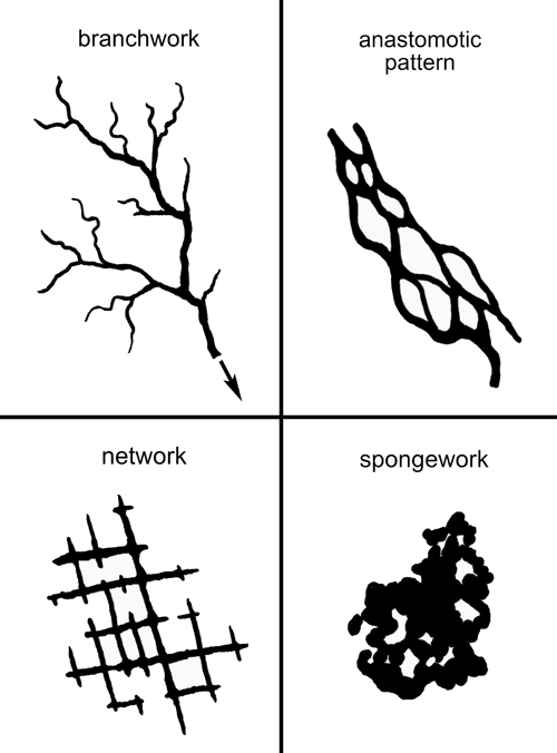
So these 4 cave patterns account for 82% of caves by number and 93% by aggregate cave length. (Stating this the other way around, all other cave patterns only account for 18% of caves by number and 7% by aggregate cave length.)

Mammoth Cave in Kentucky and Jewel Cave in South Dakota are the 1st and 3rd biggest cave systems in the world by length.

Mammoth Cave has a surface area of 80 square miles, it runs 407 feet deep, but the underground cave network is a whopping 405 miles long! In another thread, I mentioned how Mammoth Cave and a 1975 D&D game were the dual inspirations for the Colossal Cave Adventure – the first computerized interactive fiction game.

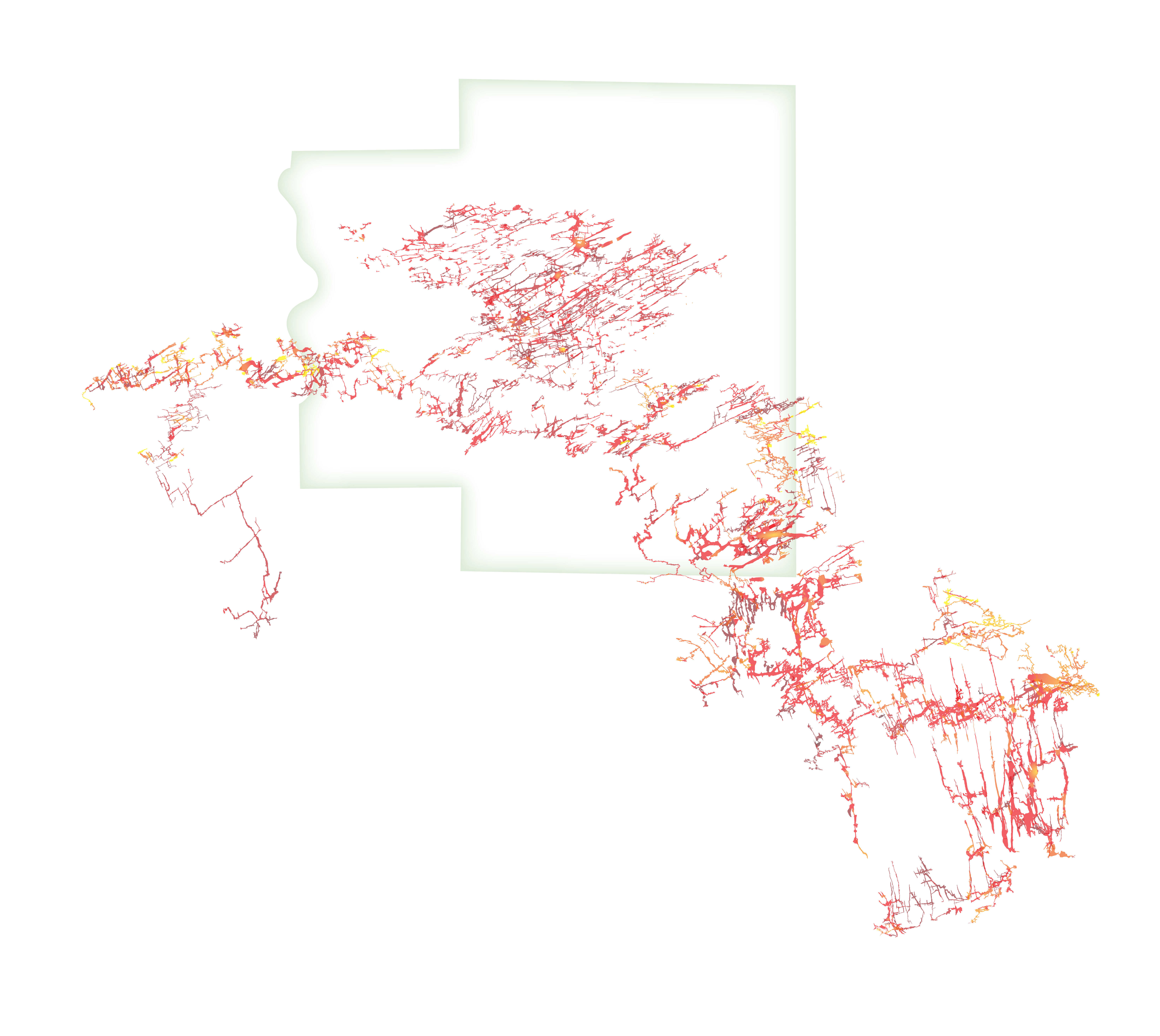
Jewel Cave is 182 miles long and 723 feet deep. Here is a map of Jewel Cave from the National Park Service – click here to see more detail (5,996px × 5,354px, 1.8MB jpg). You can see it has a dendritic pattern:

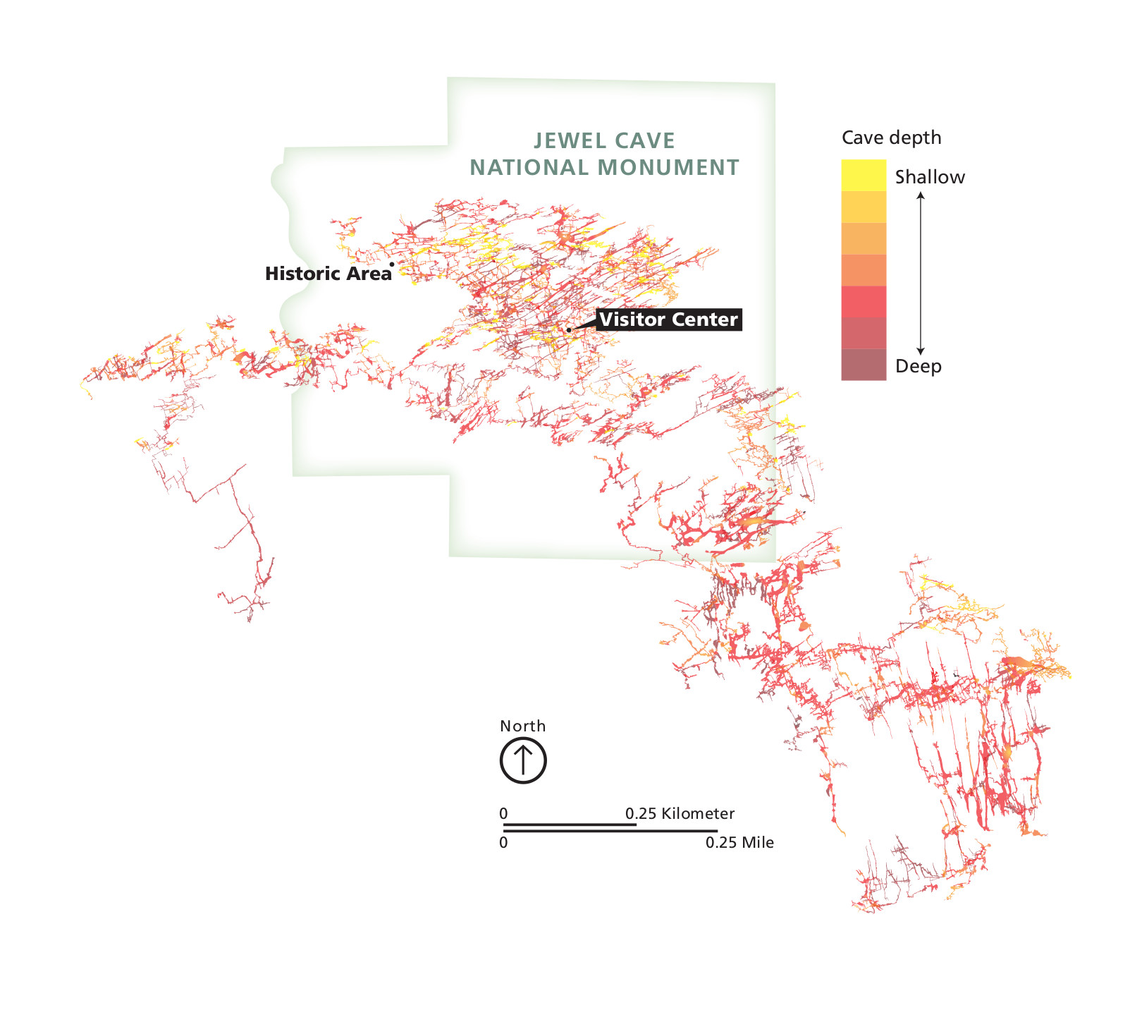
Loops occur where streams diverge and and meet again further downstream. This occurs because the chemical composition of the rock varies from place to place, and the chemical composition of the water varies over place and time. In some areas and at certain times, you’ll have microbes that take \(CO_2\) out of the water; at other places and times, they’ll add more \(CO_2\) to the water, making it more acidic; and some microbes generate \(SO_2\) instead of \(CO_2\), which creates sulfuric acid, \(H_2O + SO_2 \longrightarrow H_2SO_3\), a very strong acid.

In sum, most caves are formed by fluid flow. So the same equations that govern fluid flow also govern speleogenesis. Except that the parameters in these differential equations vary over place and time with differences in geochemistry and biochemistry. Therefore, you could generate random dungeons by simulating laminar and turbulent flow of acids over rocks. But I can’t recommend this method for generating random dungeons on the fly for tabletop use.

4.2 Mining and man-made caves

In the middle ages, castles were built from sandstone blocks. Sandstone is one of the most common minerals in the earth’s crust. And it’s soft enough to be carved into blocks with hand tools. But in order to “glue” the sandstone blocks of a castle together, engineers in the middle ages made lime mortar out of a slurry of water and kiln-fired lime. In addition, they whitewashed the sandstone with limewash. (I wrote about the real-life time and cost of constructing a castle in the thread on Building the Stronghold- calculating time.)

Even further back, the Egyptians and Romans made lime cement. In 2006, scientists used a scanning electron microscope and found that the air bubbles in the stone blocks used in the Pyramids did not occur naturally in quarried limestone, a blow to the old theory that these stones were quarried and dragged into place, and a boost the new theory that the stones were cast from lime cement.

All of these uses for limestone created a high demand for it. When ancient and medieval people wanted to construct a cathedral or a castle, they used lime from local sources within 3-5 miles, because the cost of transporting it was so high. They would use hand tools to dig mines and pits (quarries). They dug by candle light. They used child labor and unskilled labor to do the initial work of carving out the stone, which would then be finished by a skilled stonemason. Here’s a map of the Beer Quarry Caves in Devon. There is a triangular loop in the north side. The south side is just one big chamber help up with columns:

When exploring caves or quarrying rocks, people noticed veins of precious ores (gold, silver, copper) and metals useful for construction (like lead). They would dig out these veins, creating new mines.

Mining is very difficult and dangerous work. It risks:

• tunnel collapse
• releasing toxins into the air, soil, and water

Miners do back-braking work for little compensation; they develop poor health; and they often die young.

4.3 Teratogenesis

Due to the dangers posed by mining, it’s easy to imagine that in a medieval fantasy setting, warriors, wizards and clerics would create a cheap and disposable mining workforce – troglobites. It’s also easy to imagine that these cave-dwelling slaves would grow to resent their human masters and would rebel. At least that’s how I imagine monsters got their start.

Because many caves have small passages, many races of monster would be smaller than humans, like goblins; but because it is also necessary to drag large stones, some monsters would be huge, like ogres. Living and working in dark caves, most monsters have infravision. Due to their struggle against their former human slave masters, monsters hate Law and side with Chaos. Since their main skill is quarrying stones and mining ores, monsters are experts at cave construction.

Monster-made caves are much more intricate than natural caves or man-made mines. Monster lairs have an abundance of loops and labyrinths and traps to confuse and catch human trespassers.

4.4 Randomly-Generating Branchwork Patterns

Okay. Maybe I’ve convinced you that a genuine branchwork pattern cave/chasm/stream would be a cool addition to your dungeon… How does one randomly generate such a thing? We’re going to build it as a tree as follows:

1. Let \(N\) be the Strahler number of the network. Pick something manageable: 4 or 5.
2. Start with the root node. Call it \(i\). Give it Strahler number \(\omega(i)=N\). Remember that nodes (not edges) represent a cavern in a cave, a crevasse in a chasm, or a stretch of stream in a river.
3. If node \(i\) has Strahler number \(\omega(i)=1\), then it has no children – it is a leaf node, and there’s nothing left to do down this branch. Otherwise, \(i\)’s Strahler number is \(\omega(i)>1\), and \(i\) must have 2-5 children. Roll d4+1 (or d6, rerolling on 1 or 6) to determine how many children \(i\) has.
4. Roll one d6 to choose between the following two cases:
   1. Case (1-3): Two of \(i\)’s children have Strahler number \(\omega(i)-1\), and the rest have Strahler number \(1,\ldots,\omega(i)-1\) (choose at random)
   2. Case (4-6): One child has the same Strahler number as \(i\), namely \(\omega(i)\), one has Strahler number \(\omega(i)-1\), and the rest have Strahler numbers \(1,\ldots,\omega(i)-2\) (can’t be less than one; choose at random).
5. Recurse on steps (3-5) for each of \(i\)’s children.

Here’s an illustration from Wikipedia of a tree obeying these rules. The nodes are labeled with their Strahler number.

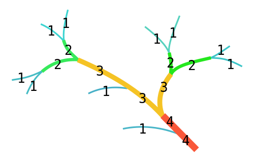
Denote by \(N(\omega)\) the number of nodes with Strahler number \(\omega\).

\(\frac{N(\omega)}{N(\omega+1)} = R_B\)

The number \(R_B\) is called the bifurcation ratio and it ranges from 2 to 5, by design.

4.4.1 Length

Denote by \(L(\omega)\) the mean length of nodes with Strahler number \(\omega\). Then

\(\frac{L(\omega+1)}{L(\omega)} = R_L\)

is called the length ratio, and it ranges from 1.5 to 3.5. So you can assign a reasonable length \(L\) to your leaf nodes (\(\omega=1\)), and then assign lengths \(L(\omega+1)=(L(\omega)) (2.5+\frac{2dF}{2})\) to nodes with higher Strahler numbers.

4.4.2 Area

There’s a similar law that governs area:

\(\frac{A(\omega+1)}{A(\omega)} = R_A\)

In this case, \(R_A\) ranges from 3 to 6. You could simulate areas for nodes with higher Strahler numbers using \(A(\omega+1)=(A(\omega)) (4.5+\frac{3dF}{2})\). Once you determine area and length, you just need to compute width=area/length.

4.4.3 Slope

Slope follows a similar law to length and area. Keep in mind that water flows downhill. The leaves have the steepest slope – they may be vertical. The root node is the most horizontal. Just to make things easy, I’d set the slope of the root node to \(S(N) = \sqrt[N]{90^{\circ}}\) and the slope of nodes with lower Strahler numbers to \(S(\omega)=S(N)^{\omega}\).

For example, in a tree with Strahler Number \(N=4\), I’d use \(S(4) \approx 3^{\circ}\), \(S(3) \approx 9.5^{\circ}\), \(S(2) \approx 30^{\circ}\), and \(S(1) \approx 90^{\circ}\).

4.4.4 Dimension

In the thread on Dreams in the Witch House, I recently posted about fractal dimensions. I don’t want to rehash any of that here. But I do want to note that stream lengths have a fractal dimension of about 1.2, and cave lengths have a fractal dimension of about 1.4.

5 Appendix: Learn You Some Graph Theory

This appendix isn’t intended as a rigorous presentation of graph theory – just a basic overview to familiarize you with some of the terminology and concepts useful for flow-chart style mapping….

A graph is a set vertices and a set of edges. An edge connects a pair of vertices.

The order of a graph is its vertex count. The size of a graph is its edge count. The degree of a vertex is the number of incident edges.

Graph theorists use specialized jargon to describe a sequence of vertices and edges in a graph. If the first vertex in the sequence is the same as the last vertex, then the sequence is closed; otherwise it’s open:

Some more terminology: A loop is an edge that connects a vertex to itself. N.B. What we were calling a “loop” geologically is called a “cycle” graph-theoretically.

Multi-edges are two or more edges between the same pair of vertices. In a directed graph, edges have a direction (like a one-way door); otherwise, it the graph is undirected. Simple graphs are undirected graphs without loops or multi-edges. Multi-graphs have multiedges, but no loops. Pseudographs have multi-edges and loops. Connected graphs have a path between every pair of vertices. Disconnected graphs have more than one component. A tree is a connected acyclic graph. A forest is an acyclic graph (“forest” usually implies it is disconnected, i.e., a forest has several components, each of which is a tree).

There are \(2^{\binom{V}{2}}\) possible simple graphs of order V. The mean degree of a vertex in a graph of order V and size E is \(\overline{deg} = \frac{2 E}{V}\).

Planar graphs are graphs that you can draw in a 2D plane without edge crossings. There are many ways to draw a planar graph, and one specific drawing of a planar graph is called a plane graph. Tutte’s spring theorem says that you can draw any planar graph with straight edges. The regions enclosed by a planar graph are called its interior faces; and the region surrounding the planar graph is its exterior (or infinite) face. Euler discovered the following relationship for a planar graph. Let:

• V = the order of the graph
• E = the size of the graph
• F = the number of faces (interior and exterior)
• C = the number of connected components of the graph

Then Euler’s formula says that for a planar graph

\(V - E + F - C = 1\)

For planar graphs, \(E \leq 3 V - 6\).

For trees, \(E = V - 1\) and \(F = 1\).

A path graph \(P_n\) is a tree with \(n\) vertices, \(n-1\) edges, exactly two leaves (i.e., vertices of degree 1), and all other vertices degree 2. Here is \(P_5\):

The number of independent cycles \(R\) in an undirected graph is given by

\(R = E - V + C\)

This number \(R\) goes by many names:

• circuit rank: \(R\)
• cyclomatic number
• nullity
• first Betti number: \(b_1\)
• dimension of the first Homology group: \(\dim H_1\)

\(R\) provides a very easy way to detect cycles in undirected graphs.

Cycle detection in graphs has important real-life applications, e.g., detecting “fake news” in social media and finding arbitrage pricing in trade networks.

The adjacency matrix of a graph with V vertices is the \(V \times V\) matrix A such that \([A]_{ij} = 1\) if there is an edge from vertex \(i\) to vertex \(j\) and 0 otherwise. The incidence matrix of a graph with V vertices and E edges is a \(V \times E\) matrix M such that \([M]_{ij} = 1\) if edge \(j\) is incident to vertex \(i\) and 0 otherwise. The degree matrix of a graph with V vertices is the \(V \times V\) matrix D such that \([D]_{ij}\) = the degree of vertex \(i\) if \(i=j\) and 0 otherwise. It is possible to use linear algebra to compute the number of connected components \(C\), the circuit rank \(R\), the number of walks from vertex \(i\) to vertex \(j\) in \(s\) steps, and other properties of a graph from the matrices A, M, and D.

You can do calculus on graphs: discrete exterior calculus. Stokes’s theorem works on graphs: \(\int_M d\omega = \int_{\partial M} \omega\). And there are graph analogs of grad, curl and div that preserve their properties, e.g., \(\text{curl} \circ \text{grad} = 0\) and \(\text{div} \circ \text{curl} = 0\).

The cycle graph on \(n\) vertices is denoted \(C_n\). It has \(n\) vertices and \(n\) edges, and every vertex has degree 2. Here is \(C_5\):

The wheel graph \(W_n\) consists of a single vertex connected to all the vertices of \(C_n\). Here is \(W_4\):

A subgraph of a graph is a subset of vertices and edges; the vertex subset must include all of the endpoints of the edge set.

Two graphs are isomorphic if they have the same structure: there is a one-to-one incidence preserving correspondence between the vertices and edges in one graph and the vertices and edges in the other graph.

The subdivision of an edge with endpoints \((u,v)\) is obtained by removing the edge \((u,v)\), adding a new vertex \(w\), and adding two edges \((u,w)\) and \((w,v)\). A graph subdivision is obtained through one or more edge subdivisions. Two graphs F and G are homeomorphic if there is an isomorphism from a subdivision of F to a subdivision of G.

A complete graph has an edge between every pair of vertices. A complete graph on \(n\) vertices is denoted \(K_n\). For example, \(K_1\) is the graph with exactly one vertex and no edges. \(K_5\) is called the pentatope graph, and it is the smallest non-planar graph:

A bipartite graph is a graph whose vertices may be partitioned into two sets A and B such that all edges have one endpoint in A and the other in B. A complete bipartite graph has an edge from every vertex in A to every vertex in B. If the vertex counts of A and B are m and n, then it is denoted \(K_{m,n}\). The graph \(K_{1,n}\) is called a star. The graph \(K_{1,3}\) is called a claw. And the graph \(K_{3,3}\) is called the utility graph. \(K_{3,3}\) is non-planar:

Kuratowski’s Theorem: A graph is planar if and only if it has no subgraph that is a subdivision of \(K_5\) or \(K_{3,3}\). Equivalently, a graph is non-planar if and only if it has a subgraph homeomorphic to the pentatope graph or the utility graph.

A spanning tree of an undirected graph is a subgraph that is a tree which has all of the vertices, but with minimum possible number of edges; it is not necessarily unique.

The complement of a graph is obtained by exchanging edges and non-edges. The complement of graph G is usually denoted with an overline/bar/macron: \(\bar{G}\). A cograph is a graph that can be generated from the single-vertex graph \(K_1\) by complementation and disjoint union.

The dual \(G^*\) of a planar graph \(G\) is defined so that \(G^*\) has a vertex wherever \(G\) has a face, and \(G^*\) has an edge wherever two faces of \(G\) are separated by an edge. The dual of a simple graph may be a pseudograph. The dual may not be unique when the planar graph has several plane graphs. A graph that’s isomorphic to its dual is called self-dual. Wheel graphs are self-dual. The following correspondence exists between the vertex counts, edge counts and face counts of planar graphs and their duals:

\(\begin{aligned}V^* = F \\E^*=E \\F^*=V\end{aligned}\)

Therefore, for a connected (i.e., \(C=1\)) simple graph, Euler’s formula implies

\(V - E + F = 2\)

and

\(V^* - E^* + F^* = 2\)

Besides subdivision, complementation and dual, there are many other operations that may be performed on graphs, e.g., vertex and edge addition and subtraction; products of graphs; edge contraction (the inverse of subdivision); and finding the line graph of a graph.

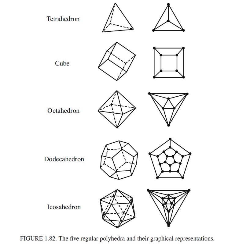
A convex regular polygon has all sides equal and all interior angles equal. A Platonic Solid is a polyhedron whose faces are all identical convex regular polygons. Each polyhedron has an associated planar graph, called a polyhedral graph or polyhedra. The following illustration (excerpted from here) shows the 5 Platonic solids and their associated planar graphs. You can use Euler’s formula to prove that there are only 5 Platonic solids.

Here is a table summarizing some important graph-theoretic properties of the 5 Platonic Solids:

Beyond graphs. You can make graphs more abstract by allowing edges to connect any number of vertices. This leads to abstract simplicial complexes and hypergraphs. Graphs are 1-D topological manifolds, with a 0-D topological invariant (number of connected components) and a 1-D topological invariant (number of independent cycles). Abstract simplicial complexes also have higher dimensional topological invariants: 2-D (number of “bubbles” or “voids”) and so on. You compute these topological invariants using a branch of linear algebra called homology. This has important applications in tomography (e.g., CAT scans and MRIs) and other kinds of image analysis.

5.1 Example: The House Graph

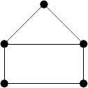
Property		Value
Order / vertex count	V	5
Size / edge count	E	6
Faces	F	3
Connected components	C	1
Euler’s formula	V - E + F - C = 1	True
Number of independent cycles	R = E - V + C	2
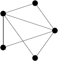
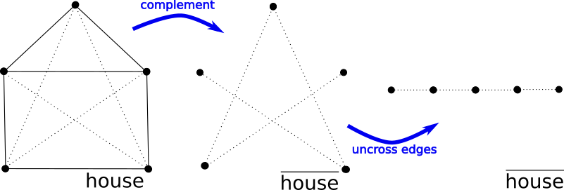
Complement	\(\overline{\text{house}} = P_5\)

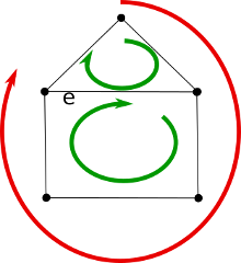
The following illustration labels the graph’s three faces: Face-1 and Face-2 are interior. And Face-3 is exterior.

The following illustration shows all the cycles in the graph. Note that there are three cycles: One around the edges surrounding each of the two interior faces (in green) plus a third around the exterior face (in red). With the given orientations, the green cycles traverse edge \(e\) in opposite directions, so that they cancel each other out along this edge when we add them, resulting in the red cycle. So, only two of the three cycles are independent – the red cycle around the exterior face is the sum of the green cycles around the two interior face. Thus, the house graph has circuit rank \(R=2\).

Here is an illustration showing how to construct its graph complement, \(\overline{\text{house}} = P_5\). Non-edges are shown in dotted lines:

Finally, here is an illustration showing how to construct its dual, \(\text{house}^*\). The dual’s vertices are shown as squares, and its edges are shown as dotted lines. Notice it’s a multigraph:

You can find out more about the house graph at WolframAlpha.

6 Document Information

This is version 0.5 (Monday, May 8, 2017).

The following 6 images were excerpted from external sources for commentary and educational use: maze generation, cave patterns, jewel cave, beer quarry caves, Strahler number (tree), Platonic Solids. In the text, I’ve linked the sources of these images.

The HTML version uses pandoc.css and MathJax.

With these limited exceptions, the remainder of the document is public domain, and you may use it or any part of it any way you see fit.

You can find this document online in several formats:

• HTML
• PDF
• Markdown
• Zip - contains all versions and source code